Circos

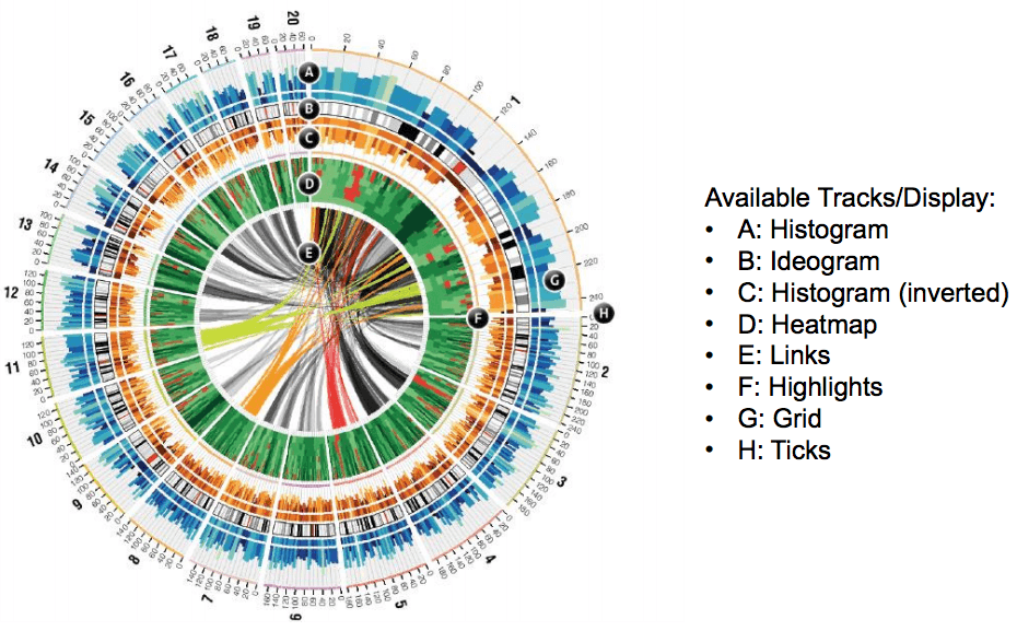
circos 是一个关系可视化圈图表达软件，常被用来绘制环状的细菌染色体或质粒，或作为可视化比较基因组学研究多个细菌基因组之间差异的工具。circos 的优点是生成的图形优美，可以表示各种类型的数据。但是缺点在于牵涉内容过于繁杂，采用的术语名称的含义往往让人摸不着头脑。教程也不够明确。circos 的目的是绘制图形，有点类似Photoshop，它提供的是工具，而不是一步速成的获得某种图形的方法。在它的圈图体系中，各种 tracks 可以分成一下一种表现图示：

• Histogram 直方图
• Ideogram 染色体示意图
• inverted Histogram 反向直放图
• Heatmap 热力图
• Links 关系线
• Highlights 加亮图示
• Ticks 圈图标尺
• Grid 圈图网格

以mit的circos图为例，可以看出一个circos绘制的圈图中可以包含什么类型的图示。

绘制一个circos图时，首先要考虑的是如何理解并展示复杂的数据关系。通过不同维度来解析数据，

$ circos -conf circos.conf

本节利用circos来简单演示几个可能会用到病原微生物成图功能。

1.安装 circos

1.1 安装依赖包

# install gd2-xpm development library
~$ sudo apt-get install libgd2-xpm-dev

# link circos perl import path. circos use "#!/usr/env perl" instead of "/usr/bin/env" which is default in ubuntu
~$ sudo ln -s /usr/bin/env /bin/env

# install perl modules needed in circos
~$ sudo cpan install Clone \
> Config::General \
> Font::TTF \
> List::MoreUtils \
> Math::Bezier \
> Math::VecStat \
> Math::Round \
> Params::Validate \
> Readonly \
> Regexp::Common \
> Set::IntSpan \
> Text::Format \
> GD \
> Statistics::Basic

1.2 安装circos

# download circos and extract
~$ wet http://circos.ca/distribution/circos-0.69.tgz
~$ tar xfz circos-0.69.tgz -C ~/apps/circos

# add circos to system
~$ sudo ln -s ~/apps/circos/bin/circos /usr/local/sbin/circos

# or you can add to your personal environment
~$ export PATH=$HOME/apps/circos/bin/
~$ circos -v

如果屏幕打印出以下信息，说明你可以正常使用circos了。

circos | v 0.69 | 6 Dec 2015 | Perl 5.018002

如果cpan下载很慢或者无法连接，可以修改mirror来改善。如果你的CPAN是安装在个人用户环境里，将~/.cpan/CPAN/MyConfig.pm文件里的urllist行后面的内容修改成离自己最近的镜像站点，比如：

'urllist' => [q[http://mirrors.sohu.com/CPAN/]],

2.配置文件

circos主要需要2类文件，一类是可视化结果的数据文件，一类是用于告诉circos如何展示的配置文件。

2.1 数据文件

由于circos只是画图工具，因此你图中要展示的数据需要自己预先准备好。比如基因组的GC含量，需要用其他程序先生成以下这种类型的文本格式文件。

染色体 开始位置 结束位置 颜色值 其他选项[可选]
chr1  1000    2000   red

2.2 配置文件

一般绘图需要以下配置文件：

• circos.conf
• ideogram.conf
• ticks.conf
• image.conf
• highlight.conf
• colors_fonts_patterns.conf

你可以将配置文件内容全部放在circos.conf里，也可以分离成单独的文件通过include方式导入。

2.2.1 circos.conf

这是circos主配置文件，其他的配置文件可以通过include的方式来导入。

<<include your_other_configure.conf>>

2.2.2 ideogram.conf

2.2.3 image.conf

2.2.4 highlight.conf

2.2.5 ticks.conf

2.3 可视化的组成要素

变量分为 Global 和 Local，对发挥作用的区块起作用。如果是某个变量在多个block中都重复使用，那么可以设置成 global 的参数，当某个block要使用新的值时，再用 local 的参数覆盖即可。

2.3.1 ideogram

2.3.2 highlights

2.3.3 ticks

2.3.4 label

2.3.5 links

2.3.6 circos.conf 参数

# 染色体的数据集
karyotype = data.txt
# 定义圈图标尺
chromosomes_units = 1000
# 如果设置成yes，所有ideogram上都会现实ticks
chromosomes_display_default = yes

2.3.7 完整circos配置文件结构

# ---- 定义图的颜色信息 ---- #
<colors>
</colors>

# ---- 定义图的字体信息 ---- #
<fonts>
</fonts>

# ---- 定义填充模式图 ---- #
<patterns>
</patterns>

# ---- 图像的基本设置信息 ---- #
<image>
</image>

# ---- ideogram 图 ---- #
<ideogram>
  <spacing>
    ideograms之间的间隔
    <pairwise>
      ideograms对（如人染色体）之间的距离
    </pairwise>
  </spacing>
</ideogram>

# ---- 标尺信息 ---- #
<ticks>
  <tick>
    各个tick的配置
  </tick>
</ticks>

# ---- 区域的放大缩小信息 ---- #
<zooms>
  <zoom>
  </zoom>
</zooms>

# ---- highlights 数据 ---- #
<highlights>
  <highlight>
    <rules>
      <rule>
        某一个具体 data track 的配置修改
      </rule>
    </rules>
  </highlight>
</highlights>

# ---- Data tracks 数据 ---- #
<plots>
  <plot>
    <rules>
      <rule>
        某一个具体 data track 的配置修改
      </rule>
    </rules>
    <axes>
      <axis>
        plot 的半径轴
      </axis>
    </axes>
    <backgrounds>
      <background>
        plot 的背景设置
      </background>
    </backgrounds>
  </plot>
</plots>

# ---- links 数据 ---- #
<links>
  <link>
    <rules>
      <rule>
        某一个具体 link 数据的配置修改
      </rule>
    </rules>
  </link>
</links>

2.3.8 circos配置的单位概念

一共有4种单位：p, r, u, b

• p表示像素，1p表示1像素
• r表示相对大小，0.95r表示95% ring 大小。
• u表示相对chromosomes_unit的长度，如果chromosomes_unit = 1000，则1u就是千分之一的染色体长度。
• b表示碱基，如果染色体长1M，那么1b就是百万分之一的长度。

3.用circos来绘图

3.1 绘制环状 Salmonella LT2 基因组

之前的教程里介绍了用DNAPlotter绘制一个基因组完成图的圈图，圆圈内容strand，GC content和GC skew。从某个角度上看，DNAplotter的配置文件与circos有一定的类似，2个软件的区别在于前者专注于绘制单个细菌基因组，后者可以完成更多的功能。第一个例子我们通过用circos来绘制类似DNAplotter生成的基因组圈图，从而学习circos的基本用法，

3.1.1 准备数据文件

从NCBI上下载Salonella LT基因组数据文件。

~$ esearch -db nuccore -query "NC_003197.1[accn]" | efetch -db nuccore -format fasta > LT2.fasta
~$ esearch -db nuccore -query "NC_003197.1[accn]" | efetch -db nuccore -format gb > LT2.gb

绘制circos所需要的ideogram所需要的几类数据，我们通过一个python脚本get\_circos\_data.py来获得。

# -*- utf-8 -*-
from Bio import SeqIO


rec = SeqIO.read("LT2.gb", "genbank")

forward = []
reverse = []

for feature in rec.features:
    if feature.type != 'gene':
        continue

    if feature.strand == 1:
        forward.append((int(feature.location.start), int(feature.location.end)))

    elif feature.strand == -1:
        reverse.append((int(feature.location.start), int(feature.location.end)))

def get_forward_strand(strands):
    """
    Create forward strands
    """
    with open("forward.txt", "w") as f:
        for strand in strands:
            f.writelines("chr1\t%d\t%d\tfillcolor=chr4\n" % (strand[0], strand[1]))

def get_reverse_strand(strands):
    """
    Create forward strands
    """
    with open("reverse.txt", "w") as f:
        for strand in strands:
            f.writelines("chr1\t%d\t%d\tfillcolor=chr6\n" % (strand[0], strand[1]))

def calc_GC_content(seq):

    """
    Return GC content of input sequence
    """

    gc = sum(seq.count(x) for x in ['G','C','g','c'])
    gc_content = gc/float(len(seq))
    return round(gc_content, 4) 

def calc_GC_skew(seq):

    """
    Reuturn GC skew of input sequence
    """

    g = seq.count('G') + seq.count('g')
    c = seq.count('C') + seq.count('c')

    try:
        skew = (g - c)/float(g + c)
    except ZeroDivisionError:
        skew = 0
    return round(skew, 4)


window = 10000
step = 5000
seqs = SeqIO.parse("LT2.fasta", "fasta")

for seq in seqs:
    seq_1 = seq.seq

with open("gc_skew.txt", "w") as f1:
    with open("gc_content.txt", "w") as f2:
        for i in range(0, len(seq_1), step):
            subseq = seq_1[i:i+window]
            gc_content = (calc_GC_content(subseq))
            gc_skew = (calc_GC_skew(subseq))
            start = (i + 1 if (i+1<=len(seq_1)) else i)
            end = ( i + step if (i+ step<=len(seq_1)) else len(seq_1))

                f1.writelines("chr1\t%d\t%d\t%s\n" % (start, end, gc_skew))
               f2.writelines("chr1\t%d\t%d\t%s\n" % (start, end, gc_content))


get_forward_strand(forward)
get_reverse_strand(reverse)

运行脚本：

~$ python get_circos_data.py

3.3.2 配置文件

建立circos.conf配置文件

~$ mkdir circos_data && cd circos_data
~/circos_data$ touch circos.conf

大部分细菌的基因组都是单染色体的，因此一个细菌基因完成图可以用1个完整的圈来表示。通过设置spacing来去除间断。

<spacing>
  default = 0u
  break = 0u
</spacing>

circos.conf 文件添加以下内容

<<include colors_fonts_patterns.conf>>

<ideogram>
 <spacing>
  default    = 0u
  break        = 0u
 </spacing>
 radius        = 0.85r
 thickness    = 5p
 stroke_thickness    = 1
 stroke_color = black
 fill = yes
 fill_color = black
</ideogram>

<image>
dir   = . 
file  = circos.png
png   = yes
svg   = yes

# radius of inscribed circle in image
radius = 1000p

# by default angle=0 is at 3 o'clock position
angle_offset = -90

#angle_orientation = counterclockwise

auto_alpha_colors = yes
auto_alpha_steps  = 5
background = white
</image>

karyotype = data/node.txt
chromosome_units = 1000
chromosomes_display_default = yes
show_ticks             = yes
show_tick_labels     = yes
show_grid            = no
grid_start            = dims(ideogram,radius_inner) - 0.5r
grid_end            = dims(ideogram,radius_inner)


# --------------------- ticks start --------------------- #

<ticks>
# if yes, skip of label of 0bp
skip_first_label = no
# if yes, skip of lable of last
skip_last_label = no

# ticks radius to show, outside or inside
radius    = dims(ideogram,radius_outer)

# genome size * label_multiplier = label units
label_multiplier = 1e-6

tick_separation = 2p
min_label_distance_to_edge = 0p
label_separation = 5p
# label distance to ticks
label_offset     = 5p
label_size = 8p
size = 20p

<tick>
spacing         = 10000u
color             = gray
show_label      = no
thickness         = 1p
</tick>

<tick>
spacing         = 100000u
color             = black
show_label      = yes
label_size        = 16p
thickness         = 2p

# label format, %.1f = 1.1, %d = 1, %.2f = 1.10
format            = %.1f
grid             = yes
grid_color        = white
grid_thickness    = 1p
</tick>

<tick>
spacing         = 1000000u
size             = 30p
color             = black
show_label      = yes
label_size        = 24p
thickness         = 3p
# label format, %.1f = 1.1, %d = 1, %.2f = 1.10
format            = %d
# plus Mb to lables
suffix            = " Mb"
grid             = yes
grid_color        = dgrey
grid_thickness    = 1p
</tick>
</ticks>
# --------------------- ticks ends ---------------------- #

# --------------------- plot start ---------------------- #
<plots>

<plot>
type  = tile
file  = data/forward.txt
r1    = 0.95r
r0    = 0.90r
margin = 1b
stroke_thickness = 0
color = orange
orientation = center
# tile height
thickness = 20p
# different layer index height
padding = 5p
layers = 1
<rules>
<rule>
condition = var(size) > 5kb
color = black
</rule>
</rules>
</plot>

<plot>
type  = tile
file  = data/reverse.txt
r1    = 0.92r
r0    = 0.87r
margin = 1b
stroke_thickness = 0
color = blue
thickness = 20p
padding = 5p
# display one layer of plot
layers = 1
<rule>
condition = var(size) > 3kb
color = black
</rule>
</plot>

<plot>
type = line
r1 = 0.85r
r0 = 0.75r
file = data/gc_skew.txt
thickness = 1
max_gap = 1u
color   = vdgrey
# max/min value of line plotting
min     = -0.15
max     = 0.15
fill_color = vdgrey_a3
<backgrounds>
<background>
color     = vvlgreen
y0        = 0.05
</background>
<background>
color     = vvlred
y1        = -0.05
</background>
</backgrounds>

<axes>
<axis>
color     = lgrey_a2
thickness = 1
spacing   = 0.04r
</axis>
</axes>
</plot>

<plot>
type = histogram
r1 = 0.70r
r0 = 0.60r
file = data/gc_content.txt
thickness = 1
max_gap = 1u
min     = 0
max     = 1
<rules>
<rule>
condition = 1
fill_color = eval(sprintf("spectral-9-div-%d", remap_int(var(value), 0,1,1,9)))
</rule>
</rules>
</plot>

</plots>

<<include housekeeping.conf>>

3.2 绘制测序拼接结果信息

3.2.1 数据准备

3.2.2 配置文件

3.3. 绘制一个比较基因组学数据

BRIG 常被用来绘制的多个细菌比较基因组学数据。本例用circos绘制类似的圈图，通过结果可视化来发现和展示生物学信息。

3.3.1 数据准备

3.3.2 配置文件

Reference

1. Circos Official Website
2. Creating Circos Plots
3. Plot of the complete Pseudomonas pseudoalcaligenes CECT5344 genome